METHODOLOGY

ANALYSIS OF SEDIMENT SOURCES AND ESTIMATION OF SEDIMENT SUPPLY TO THE DRAINAGE NETWORK (WP1)

Landslide Mapping and Volume Characterization (Task 1.1)
A multi-temporal (1954–2020) landslide inventory has been compiled based on air photo interpretation, following the methodology outlined in [1–35] and recently adapted for clay-rich terrains in the Northern Apennines [34]. The inventories identify sediment sources and, where discernible, distinguish among initiation, transportation, and deposition zones. Landslide attributes include movement type, initiation site morphology/landform, receiving landform (sediment sink), degree of confinement in the transportation zone, material type, year of first photo-documented appearance, headscarp activity (e.g., upslope migration or revegetation), deposition lobe activity (e.g., gully incision or revegetation), and related local channel impacts (e.g., occlusion, avulsion, or bed coarsening). Geometric parameters such as area, length, and average width are also assessed.
Sediment sinks are categorized based on downstream sediment delivery potential:

• Unchannelled topography (on-site/low mobility)
• Ephemeral or seasonal channels (moderate mobility)
• Perennial channels (high mobility)

Additionally, the mapping includes geomorphic barriers such as check dams, levees, dykes, and relict landslide lobes. In the Nure/Aveto case study, the inventory includes landsliding associated with the flash floods of 2015 [33]. Field-based and UAV-assisted multitemporal surveys are carried out on selected recent landslide initiation and/or deposition zones. These support the derivation of area–depth and area–volume relationships specific to each study area [1,36]. Uncertainty are assessed by evaluating landslide visibility thresholds across varying land cover types [37,38] and by quantifying measurement uncertainties in mapped landslide areas. To test mapping consistency, inventories are replicated in selected sub-basins using different imagery sources (e.g., aerial vs. satellite), with UAV and field survey results serving as ground-truth benchmarks. This contributes to refining comparative mapping protocols, expanding on prior work conducted in the Central Apennines [39].

Susceptibility mapping (Task 1.2)
Using one subset of the inventoried debris flows initiation zones as training supporting evidence, geostatistical methods such as Weight of Evidence, Frequency Ratio and Logistic Regression, are used to derive susceptibility maps of debris flow initiation areas [40–42]. The maps are validated using a separate subset of inventoried debris flow initiation zones, employing Receiver Operating Characteristic (ROC) and Success Rate Curves [43,44]. These maps, which illustrate the spatial probability of debris flow initiation, are then integrated with magnitude data to define potential sediment source areas.

Landslide Sediment Supply to the Drainage Network (Task 1.3)
The empirical area–volume relationships derived in Task 1.1 [1,36] is applied to the basin-wide landslide inventories, enabling the conversion of mapped landslide areas—whether initiation zones, deposition zones, or susceptible areas—into estimates of mobilized debris volumes. These estimates are further evaluated through comparisons with field and UAV-derived measurements.
Field and UAV-based volume estimates are compared with gross geometric calculations (volume = length × average width × average depth) as well as Structure-from-Motion (SfM) derived volumes [45]. For recent landslides (e.g., 1–3 years old), repeated SfM surveys enable the quantification of sediment transfer processes (erosion and deposition) and surface deformation along landslide paths and their delivery into the drainage network. These processes are still poorly understood due to both theoretical limitations and a scarcity of high-resolution empirical data [46].
In most remotely-sensed inventories, landslide connectivity to the drainage network is either defined purely based on topology [3], or—when volume transfer is considered—assumes total delivery of the mobilized material [2], an unrealistic simplification. To address this, in cases such as the 2015 storm-triggered events in the Aveto/Nure basins, geomorphic change detection are conducted using DoD (DEM of Difference) analysis.
This DoD analysis are carried out in study sites where high-resolution, multi-temporal DEMs are available. Uncertainty in the DEMs and the propagation of related errors are rigorously accounted for to distinguish real geomorphic changes from noise [7,47]. The volumes of mobilized debris and the spatial patterns of erosion and deposition derived from DoD are then compared with those obtained from the airphoto-based inventories, offering an independent, high-resolution benchmark. This comparison helps refine the DoD workflow—including point cloud alignment, DEM error analysis, and filtering—and validate its application against field and UAV-derived measurements.
By integrating these findings with outputs from landslide mapping and characterization activities, we derive basin-scale volumetric rates of sediment transfer (yield) and sediment supply to the drainage network [2,37], expressed through graph theory approaches and magnitude–frequency frameworks [48].
Finally, methodological guidelines are developed to support the assessment of landslide-derived sediment supply to drainage networks. These span the full workflow—from the compilation of remotely-sensed inventories, to the planning of field surveys based on land cover and landslide types, and the selection of optimal imagery types depending on required temporal and spatial resolutions.

EVALUATING GEOMORPHIC CHANGE AND SEDIMENT TRANSFER (WP2)

Monitoring of geomorphic change and sediment transfer forms an empirical basis to calibrate the stochastic and physically-based models (WP3). Activities are performed at the landslide scar and channel reach scales. The study encompasses landslide coupled and uncoupled conditions. In order to capture and characterize intrinsic site variability associated with the different geomorphic processes involved, the rheology and grain size distribution (GSD) of the sedimentary materials, and the complexity of the boundary (submerged and subaerial) conditions, a combination of field, proximal and remote sensing techniques is adopted.
Each study reach has a station instrumented with a time-lapse camera, a water level sensor, and a geophone. The first affords direct observation of the flood conditions. The second allows constraining stage-discharge relations through salt dilution and velocimetric surveys. The third ensures continuous monitoring of seismic activity by the stream channel and is used as a proxy for bedload transport [49]. To evaluate the contribution of suspended load to total sediment transport, as well as interactions between suspended load and bedload, one station is instrumented with a turbidimeter. Rainfall and atmospheric temperature over the study area are drawn from local meteorological stations (i.e., ARPAs).

Estimating landslide to drainage transfer and sediment dynamics through proximal sensing (Task 2.1)
High-resolution 3D mapping methods are conducted via UAV-based photogrammetric and LiDAR surveys. In this context, GNSS positioning of Ground Control Points and Checkpoints guarantees geodetic reference for accurate coregistration of sequential 3D digital terrain models and orthophotos [50]. These surveys also aid in characterizing the boundary conditions (i.e., surficial grain size distribution (GSD), surface roughness and slope gradient) of the study reaches before bedload monitoring. In particular, remotely-based GSD characterization is complemented by direct pebble count and bulk sampling on the channel bed [51] to assess armoring ratios and critical hydraulic thresholds for channel instability.

Bedload monitoring in coupled and uncoupled conditions (Task 2.2)
Bedload transport, which controls topographic and morphologic changes in mountain streams, is monitored by particle tracking approaches, in conjunction with multi-temporal topographic information derived from the UAV surveys described above, and continuous seismic monitoring at the instrumented stations. Tracking of pebble- to cobble-sized particle dynamics employs RFID [29]. This technique, performed with a handheld reader and GNSS receiver during post-flood surveys, yields particle travel distance and burial depth as a function of tracer size. In turn, this information is used to derive active channel width and depth, as well as the virtual velocity of different particle-size classes, which finally leads to estimates of sediment volumes transported between sequential field surveys [52].
Simultaneously, volumetric estimation of channel-reach aggradation and degradation is obtained through thresholded DoD analysis of the UAV-derived DSMs [7]. This estimate complements the volumetric transport rates obtained through particle tracking, allowing refinement of the sediment budget between sequential surveys. Finally, analysis of continuous seismic monitoring allows characterizing within-flood bedload dynamics in relation to antecedent flooding history and hydrograph shape.

Suspended load monitoring through remote sensing: testing and empirical calibration (Task 2.3)
Few studies estimate suspended sediment concentrations (SSC) along rivers from space [53], highlighting the challenges in validating these remotely-sensed products with on-site empirical measurements [54]. In situ measurements [55,56] allow developing and validating models for analyzing inland waters from remotely sensed data. As inland waters are characterized by high spatial and temporal variability, remote data have to be collected simultaneously and in proximity to the monitoring stations [54].
In this context, the first step involves verifying the most widely used measurement protocols (e.g., NASA protocols), in order to select those applicable to the currently available EO products, while guaranteeing the needed accuracy, level of confidence, and compatibility. Field-based SSC data are collected at different time intervals in correspondence with remote data acquisitions and under varying river conditions. Proximal multispectral data are compared to optical satellite data to evaluate the suitability and effectiveness of different platforms (e.g., Sentinel-2) in retrieving SSC. Possible advantages in classification and estimation of suspended load may arise from the use of spectral indices like NDWI (Normalized Difference Water Index) [57], or alternative indices.

MODELING SEDIMENT TRANSPORT AND CONNECTIVITY (WP3)

In this work package, we start with the assessment of structural (potential) sediment connectivity, through the application of a geomorphometric index, and continue with the modeling of sediment transport and functional connectivity at the drainage network (i.e., CASCADE) and at hillslope/basin (i.e., LANDPLANER, MPM) scales.

Structural sediment connectivity assessment (Task 3.1)
This task aims at testing geomorphometric GIS-based indices for the identification and characterization of hillslope sediment delivery potential, hence spatial patterns of sediment connectivity. These analyses are useful for constraining geomorphometric thresholds of landslide initiation, transport, and deposition, including geomorphic barriers impeding downslope/stream sediment transfer.
We start with the semi-automated extraction of the drainage network from LiDAR-derived and from 5-m DTMs using a range of simple-to-sophisticated algorithms (e.g., [58]), depending on DTM resolution. Drainage extraction is a critical preliminary step for implementing the modeling of sediment routing (T3.2), as well as for deriving local slope and contributing area values associated with strategic geomorphic landforms of hillslope (e.g., landslide and debris-flow initiation, transport, and deposition sites) and fluvial (e.g., channel heads, fans, terraces, and tributary confluences across ephemeral and perennial channels) dominance and transition (e.g., [59]) mapped in WP1 (Fig. 1).
We further evaluate the degree of sediment delivery to streams through the Index of sediment Connectivity (IC, [25] [26], Fig. 2), exploiting the functionality of SedInConnect [60]. Integration of IC index maps with key landforms mapped in WP1, such as landslide scars and deposition lobes, as well as colluvial and fluvial sinks (e.g., fans, terraces, and floodplains) or barriers (e.g., roads, dykes, and check-dams), allows defining IC ranges of variation (envelopes) for different types of sediment sources, sinks, and barriers in the study areas.
Such data integration allows not only evaluating which sediment sources are effectively coupled to the target channel reaches [61], but also constraining empirical relations between volumetric rates of landslide sediment supply and IC index values at the sub-basin scale. Similar relations, with relevant error bars, allow assigning an IC-based estimate of sediment supply in basins lacking landslide inventories. Finally, we compile relevant guidelines to define the methodological workflow and best practices for the IC parameters calibration, and we provide a simplified framework validated in our study basins to be used in other areas of the Northern Apennines with limited mapping information.

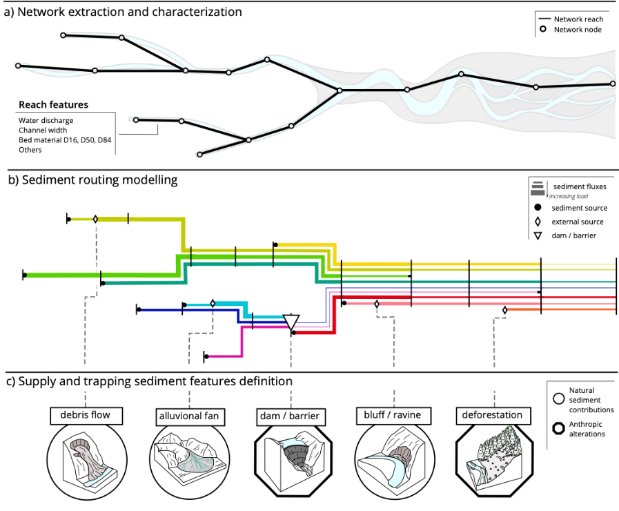
Modeling sediment transport and connectivity at the drainage network scale with CASCADE (Task 3.2)
The CASCADE model [29][30] is applied to explore basin-scale sediment connectivity using the fluvial drainage network. CASCADE provides the timing, grain sizes, magnitude, and provenance of sediment delivered to river reaches within a network. It explicitly accounts for the nexus between sediment delivery and conveyance—hence between local deposition and basin-scale sediment redistribution patterns along the fluvial drainage network.
CASCADE’s implementation (Fig. 3) involves the following tasks:

1. subdivision of the drainage network into homogeneous channel reaches
2. measurement of bankfull channel width from orthophotos and fieldwork, and generalization of drainage area–channel width empirical relations at the network scale
3. characterization of the hydrological regime of each study reach using available distributed hydrological models
4. assignment of landslide sediment supply to each study reach using the spatially distributed outputs estimated during the project

CASCADE model validation and sensitivity analysis are performed with field data collected in selected river reaches [WP2].
Surficial grain size distribution (GSD) is obtained, depending on site characteristics, via manual pebble count or UAV-based photosieving [62] (WP2).
A sensitivity analysis assesses the significance of key CASCADE parameters to model performance.
Validated CASCADE model simulations are run to assess the effects on fluvial sediment fluxes and connectivity patterns in the analyzed river networks caused by anthropogenic impacts (e.g., barrier construction/removal and channel engineering) and by realistic changes in the timing and magnitude of landslide sediment supply resulting from climatic and land cover changes.
These simulations aim to identify, under different forcing scenarios:

1. problematic reaches in terms of sediment aggradation and/or degradation—conditions that may lead to channel avulsions, bank failures, and levee breaching along the drainage network
2. the recovery time needed to attain pre-disturbance conditions or to reach a new equilibrium

Distributed modeling of sediment transport and connectivity at hillslope and basin scales with LANDPLANER and MPM (Task 3.3)
The open-source LANDPLANER model [32] is applied to explore sediment dynamics (erosion, transport, and deposition) along hillslopes and to estimate sediment export to the drainage network due to landsliding. This tool is built upon a distributed hydrological modeling procedure and uses a simplified set of input data, namely: (i) a slope and a flow accumulation map derived from a DTM; (ii) meteorological data; and (iii) a Curve Number map derived from land use/cover and soil maps based on the SCS method (https://www.nrcs.usda.gov/).

LANDPLANER primarily estimates the partition of rainfall into infiltration and runoff, and secondarily the related sediment erosion, transport, and deposition. The model is set up and calibrated under the specific conditions of the study basins using empirical data collected in WP1 and WP2. The effectiveness of calibration depends on the type, quality, and accuracy of the empirical data.

Multiple calibration approaches are tested, accounting for the presence of landslides on hillslopes and their potential sediment supply. The calibrated model is then used to estimate dynamic water and sediment connectivity in relation to rainfall and the spatio-temporal patterns of landslides, as well as to site-specific land use, vegetation, and soil conditions.

Scenario-based simulations evaluate sediment dynamics for real or plausible basin management strategies in response to varying natural and/or anthropogenic forcings (Fig. 4).

The Material Point Method (MPM) is a physically-based numerical simulation technique used to model the behavior of continuum materials, especially those undergoing large deformations, like landslides [62]. It combines the Lagrangian and Eulerian perspectives [63]. Material points (i.e., the particles) representing the landslide-prone mass, move with the material and each point carries physical state variables (e.g., mass, density, stress, strains, etc). A background grid (fixed in space) is used temporarily each time step to solve partial differential equations (PDEs) efficiently. The computed information (e.g., positions, velocities, accelerations, etc) are then transferred to the material points which updates their locations. Afterwards, the computational grid is reset (it doesn’t carry memory between time steps). These numerical features make MPM handle large deformations better than traditional finite element methods (FEMs), which instead undergo extreme and unbearable mesh distortions [63, 64].
A 2D single-phase (solid phase only) MPM model has been applied to study an earth-slide in the Sillaro river basin, by using the code developed by Soga Research Group at the University of Berkeley, California (GitHub – geomechanics/mpm: High-Performance Material Point Method). The geometry of the numerical model comprises two sub-regions: a potential moving mass composed of 6747 material points, and a fixed sub-region over which the moving mass can slide (Fig.5). The level-set and barrier method [65] is used to determine the position of each material point relative to the boundary of the fixed sub-domain and to apply a proportional force to any particle that crosses this boundary, to preserve physical consistency (Fig. 6). Input files are: (i) topography of initial state of the slope; (ii) undrained soil parameters (i.e., total unit weight, undrained Young’s modulus, undrained shear strength), (iii) initial total stress state.

References

[1] F Guzzetti et al, Earth Planet. Sci. Lett. 279: 222–229, 2009
[2] F Brardinoni et al, Earth Planet. Sci. Lett. 284: 310-319, 2009
[3] L Li et al, Landslides, 13:787–794, 2016
[4] DG Sutherland et al, GSA Bull. 114: 1036-1048, 2002
[5] P Schuerch et al, Geomorphology, 78: 222-235, 2006
[6] KB Gran & JA Czuba, Geomorphology, 277: 17-30, 2017
[7] JM Wheaton et al, Earth Surf. Process. Landf. 35: 136-156, 2010
[8] MA Hassan & P Ergenzinger, Tools Fluv. Geomorphol.:397-423, 2003
[9] H Lamarre et al, J. Sediment. Res. 75: 736-741, 2005
[10] CW Fuller et al, J. Geol. 111: 71-87, 2003
[11] TY Teng et al, Water 12:10, 2020
[12] JM Martinez et al, Catena 79: 257-264, 2009
[13] C Kuhn et al, Remote Sens. Environ. 224: 104-118, 2019
[14] R Espinoza Villar et al, J. South Am. Earth Sci. 44: 45-54, 2013
[15] RM Cavalli, Remote Sens. 12:9, 2020
[16] RM Cavalli et al, J. Environ. Manag. 90: 2199-2211, 2009
[17] DE Alexander, Geography, 65: 95-100, 1980
[18] M Cavalli et al, Sci. Total Environ. 673: 763-767, 2019
[19] J Hooke, Geomorphology 56: 79-94, 2003
[20] G Brierley et al, Area 38: 165-174, 2006
[21] KA Fryirs et al, Catena 70: 49-67, 2007
[22] LJ Bracken et al, Earth Surf. Process. Landf. 40: 177-188, 2015
[23] T Heckmann et al, Earth-Sci. Rev. 187: 77-108, 2018
[24] R Brazier et al, GRA, EGU2015, 17:15814, 2015
[25] L Borselli et al, Catena 75: 268-277, 2008
[26] M Cavalli et al, Geomorphology 188:31–41, 2013
[27] A Gay et al, J. Soils Sediments 16: 280-293, 2016
[28] JA Czuba & E Foufoula‐Georgiou, Water Resour. Res. 50: 3826-3851, 2014
[29] RJP Schmitt et al, Water Resour. Res. 52: 3941-3965, 2016
[30] RJP Schmitt et al, J. Geophys. Res. Earth Surf. 123: 2-25, 2018
[31] P Reichenbach et al, Earth-Sci. Rev. 180: 60-91, 2018
[32] M Rossi, PhD Thesis, doi:10.13140/2.1.3835.0404
[33] G Ciccarese et al, Rend. Online Soc. Geol. Ital. 41: 127-130, 2016
[34] S Pittau et al, Rend. Online Soc. Geol. Ital., 54: 17-31, 2021
[35] F Brardinoni et al, http://www.sedalp.eu/download/dwd/reports/WP4_Report.pdf
[36] IJ Larsen et al, Nat. Geosci. 3:4, 2010
[37] F Brardinoni et al, Geology, 40:455-458, 2012
[38] TR Turner et al, For. Ecol. Manag. 259: 2233–2247, 2010
[39] F Fiorucci et al, Geomorphology, 129: 59–70, 2011
[40] A Carrara et al, Geomorphology, 94: 353–378, 2008
[41] J Blahut et al, Geomorphology, 119: 36–51, 2010
[42] M Cama et al, Environ. Earth Sci. 75: 238, 2016
[43] J Corominas et al, Bull. Eng. Geol. Environ. 73: 209-263, 2014
[44] M Rossi et al, Geomorphology, 114: 129-142, 2010
[45] MJ Westoby et al, Geomorphology, 179: 300-314, 2012
[46] O Hungr & SG Evans, GSA Bull. 116: 1240-1252, 2004
[47] M Cavalli et al, Geomorphology, 291: 4-16, 2017
[48] N Hovius et al, Geology 25: 231-234, 1997
[49] C Misset et al, Geophys. Res. Lett, 48: e2020GL090696
[50] P Mora et al, Eng. Geol. 68: 103–121, 2003
[51] M Kondolf et al, Tools Fluv. Geomorphol. 347-395, 2003
[52] F Liébault & JB Laronne, Geodin. Acta 21: 23-34, 2008
[53] FJS Pereira et al, Int. J. Appl. Earth Obs. Geoinf. 79: 153-161, 2019
[54] JL Mueller et al, doi: 10.25607/OBP-63
[55] D Pavanelli & A Bigi, Biosyst. Eng. 90: 75-83, 2005
[56] DH Schoellhamer & SA Wright, IAHS Pub 283: 28-36, 2003
[57] C Qiao et al, J. Indian Soc. Remote Sens. 40:421–433, 2012
[58] M Cavalli et al, Eur. J. Remote Sens. 46:152–174, 2013
[59] DR Montgomery & E Foufoula‐Georgiou, Water Resour. Res. 29:3925–3934, 1993
[60] S Crema & M Cavalli, Comput. Geosci. 111:39–45, 2018
[61] MG Persichillo et al, Catena 160:261–274, 2018
[62] PE Carbonneau et al, Earth Surf. Process. Landf. 43:1160–1166, 2018
[63] A Yerro et al, Can. Geotech. J., 56(9):1304–1317, 2019
[64] X Zhang et al, Academic Press, ISBN: 978-0-12-407716-4, 2016
[65] J Fern et al, CRC Press, ISBN: 9780429028090, 2019
[66] LED Talbot et al, The 15th Annual MPM Workshop, 2024